Create Interesting Datasets
Noah Pollock
November 14, 2018
Scope
I needed a dataset, so I created one!
Introduction and Prerequisites
I co-taught then solo-taught the pre-conference workshop at the Michigan Association for Institutional Research in 2017 and 2018. The topic was an introduction to R. I knew I needed a dataset that would engage my audience. It had to be relevent to their work as professionals in higher education. I could have dumped some data from our database and deidentified it, but instead I thought I would cease the opportunity as a learning tool. I created my own dataset with interesting qualities. By interesting, I mean statistical effects such as mean differences between groups, variables that explain variability in other variables (and perhaps at variable levels!), and the ability to be charted and graphed in fun or useful ways.
For this post, we’ll create these datasets purely with base R
functions. However, I use ggplot2 to show how the dataset
is interesting with plots.
A few good reasons to create your own dataset:
- Mocking up visualizations
- Testing our understanding of statistics
- Simulations (e.g., probabilities or algorithms)
- Teaching
A few bad reasons:
- You didn’t get enough responses to your survey
- Your effects are too small and p-values to large to publish
The Data
We’ll create a dataset that showcases what recent college grads do after they graduate and what factors might impact their outcomes. For example, is taking advantage of the university’s career center related to post-graduation salary? Another example is whether grads with higher GPAs have higher employement rates.
The Basics
We’ll need to learn to use a few base R functions such as
sample() and rep(). If you feel confident with
these functions then you could probably skip ahead to the next
section.
To efficiently create a dataset, we want to write the smallest amount
of code as possible. That’s where sample() and
rep() come in. With sample() we can randomly
sample from a small subset of values (e.g., a validation-set) and then
we could repeat that sampling, or anything else, with
rep(). Let’s take a look.
## [1] 3 6 1# same as above except that I sample 11 times and
# every time a number is sampled it's then put back into the pool
sample(1:10,size = 11,replace = TRUE)## [1] 4 7 6 1 9 3 6 8 2 5 1# bonus, I won't run these, but try them at home!
# choose 1 to 10 random numbers from an integer vector of 1 to 10
# lapply(1:10,function(x) sample(x,size=x))
# same as above except that every time a number is sampled,
# it's then put back into the pool and could be randomly selected again.
# lapply(1:10,function(x) sample(x,size=x,replace=TRUE))## [1] 1 2 3 4 5 1 2 3 4 5# take a sample of 6 items from a pool of integers 1 to 5
# and repeat that exact sample twice
rep(
sample(1:5,size = 6,replace = TRUE),
2)## [1] 5 2 1 1 4 4 5 2 1 1 4 4# take a sample of 12 items from a pool of integers 1 to 5
# don't use repeat so that all 12 are random
sample(1:5,size = 6*2,replace = TRUE)## [1] 4 2 2 3 2 1 1 5 1 5 4 2# sample "yes" and "no" 10 times,
# encourage that sample to be %80 yes and %20 no
# repeat that exact sample twice
rep(sample(c("Yes","No"),prob=c(.80,.20),size = 10,replace = TRUE),2)## [1] "Yes" "Yes" "Yes" "Yes" "Yes" "Yes" "Yes" "No" "Yes" "Yes" "Yes" "Yes"
## [13] "Yes" "Yes" "Yes" "Yes" "Yes" "No" "Yes" "Yes"Create the Dataset
Once you understand the basics of rep() and
sample() creating an interesting dataset is fairly
straightforward. First, a simple example. Below, we force a main effect
of the experimental condition onto the dependent variable where the
Control condition exhibits far more Losses than the Experimental
condition. A Chi-Square test of independence tells us that we succeeded
in making the two variables related.
experiment_df <- data.frame(
  #independent / explanatory / predictor variable
  IV = c(rep("Control",1000),rep("Experiment",1000)),

  # dependent / response / outcome variable
  DV = c(sample(c("Losses","Wins"),prob=c(.80,.20),size = 1000,replace = TRUE),
         sample(c("Losses","Wins"),prob=c(.30,.70),size = 1000,replace = TRUE))
)

table(experiment_df) # contingency table
## DV
## IV Losses Wins
## Control 808 192
## Experiment 314 686##
## Pearson's Chi-squared test with Yates' continuity correction
##
## data: experiment_df$IV and experiment_df$DV
## X-squared = 493.44, df = 1, p-value < 2.2e-16Now a more complex and interesting example.
set.seed(100) # number generator so 'random' numbers are reproducibile
n_students <- 1000 # the number of number of grads per cohort

# five years of grads where:
  # the suffix 10 = winter semester grads
  # the suffix 40 = fall semester grads
terms <- sort(rep(c(paste0(2014:2018,"10"),paste0(2013:2017,"40")),n_students))
n_terms <- length(unique(terms)) #number of terms generated

air_df <- data.frame( # make it a dataframe
  student_id = 1:(n_students*n_terms), # arbitrary unique identifier
  term_code = terms, # assign terms as term_code

  # randomly assign one of the three schools, do it for every grad for every term
    # eg "BA" = Business Administration
  school = sample(c("BA","AS","EG"),size=n_students*n_terms,replace=TRUE),

  # randomly assign an admit code, do it for every grad for every term,
    # but repeat the same order term after term
  ATYP = rep(sample(c("F","T"),size=n_students,replace=TRUE),n_terms),

  # randomly assign a binary sex code, do it for every grad for every term,
    # but repeat the same order term after term
    # and force the porportion to be %55 Male
  sex = rep(sample(c("M","F"),prob=c(.55,.45),size=n_students,replace=TRUE),n_terms),

  # randomly assign an residency code (eg in-state), do it for every grad for every term,
    # but repeat the same order term after term
  residency = rep(sample(c("I","O"),size=n_students,replace=TRUE),n_terms),

  # number of times a grad met with career services (from 0 to 10 times)
    # force a random uniform distribution across the dataset.
  career_use = round(runif(n_students*n_terms,0,10)),

  # randomly assign a post-graduation outcome, do it for every grad for every term,
    # and force the porportion to be %64 Employed, %27 Grad School, etc
  post_grad_outcome = sample(c("Employed","Grad School","Still Seeking","Other"),prob=c(.64,.27,.07,.02),size=n_students*n_terms,replace=TRUE),

  # these vars are placeholders
  gpa = 0,
  salary = 0,

  # let the strings be chracters, not factors
  stringsAsFactors = FALSE
)

# use a linear regression equation to force relationship
  # between career_use and gpa for Freshman admits
air_df$gpa <- ifelse(air_df$ATYP=="F",
                     #intercept + slope*value + error/noise
                     #different slopes for a nice interaction effect
                     2.5 + .15*air_df$career_use + rnorm(n_students*n_terms,0,1),
                     3.7 + .01*air_df$career_use + rnorm(n_students*n_terms,0,1))
# adjust for impossible values (ie a GPA greater than 4.0 or less than zer0)
air_df$gpa = ifelse(air_df$gpa>4,runif(n_students*n_terms,3.2,4),air_df$gpa) # keep gpa under 4
air_df$gpa = ifelse(air_df$gpa<0,runif(n_students*n_terms,0,1),air_df$gpa) # keep gpa above 0

air_df$career_use <- ifelse(air_df$post_grad_outcome=="Employed",
                            #intercept + slope*value + error/noise
                            #different slopes for a nice interaction effect
                            sample(0:10
                                   ,prob=c(3:13)
                                   ,replace=TRUE
                                   ,size=length(
                                     air_df$career_use[air_df$post_grad_outcome=="Employed"])),
                            air_df$career_use)

air_df$salary <- ifelse(air_df$school=="EG",
                        #intercept + slope*value + error/noise
                        #different slopes for a nice interaction effect
                        64000 + 750*air_df$career_use + rnorm(n_students*n_terms,0,1000),
                        ifelse(air_df$school=="AS",
                               48000 + 10*air_df$career_use + rnorm(n_students*n_terms,0,4000),
                               51000 + 400*air_df$career_use + rnorm(n_students*n_terms,0,2700)))
air_df$salary <- ifelse(air_df$post_grad_outcome=="Employed",air_df$salary,NA)
Show Interest
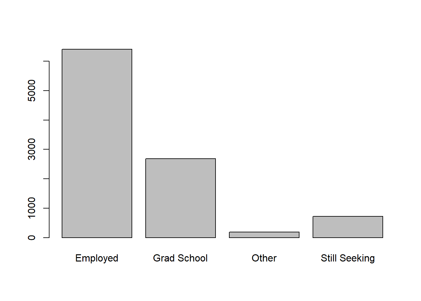
Here’s a basic plot showing the number of graduates with each
post-graduation outcome and how we forced each level to exist in a
specific proportion by specifying the prob argument in the
sample() function.
I included a report that I built with this dataset as a teaching tool at the 2018 Pre-conference for the Michigan Association for Institutional Research. Note that a few of the plots and tables below use recoded variables and two other datasets that I created as well. I included the data tidying we performed and one of the other datasets. The other dataset was a simple two column csv file with industries and counts. Eventually, I will create a blog post detailing this report.
library(dplyr)

air_df <- air_df %>%
  rename(admit_type = ATYP) %>%
  mutate(
    school_recode = recode(school,
           "AS" = "Arts and Sciences",
           "BA" = "Business",
           "EG" = "Engineering and Computer Science"),
    year = substr(term_code,1,4),
    term_type =
      ifelse(
        substr(term_code,5,6)=="10",
        "Winter",
        "Fall"),
    term_desc =
      ifelse(
        substr(term_code,5,6)=="10",
        paste("Winter",substr(term_code,1,4),sep=" "),
        paste("Fall",substr(term_code,1,4),sep=" ")),
    career_use_bin = ifelse(career_use>0,"Engaged","Did Not Engage"), #use case_when instead?
    pg_outcome_bin = case_when(post_grad_outcome %in%
                                 c("Employed","Grad School") ~ TRUE
                               ,post_grad_outcome %in%
                                 c("Still Seeking","Other") ~ FALSE
                               )
    )

roi_df <- data.frame(
  income_source = c("Minimum Wage",
                    "High School Diploma",
                    "Some College",
                    "10 Years after Attending OI",
                    "Bachelors"),
  amount = c(8.15*40*52, # source: Department of Labor Statistics
             26762, # source: https://factfinder.census.gov/faces/tableservices/jsf/pages/productview.xhtml?src=CF
             31801, # source: Census.gov ^
             43100, # source: college scorecard
             49711) # source: Census.gov ^
,stringsAsFactors = FALSE)